CFD grid set-up calculator
On this page:
- Automated definition of setttings in Star-CCM+
- Background
- Free surface mesh recomendations
- User interface
- Download and install
I am developing a web-based version of the app. At present, the web-based version of the app uses the ITTC correlation line only. I am adding further functionality. The standalone version of the webpage calculator is available here or by expanding the section below.
Web-based $y^+$ calculator
Automated definition of setttings in Star-CCM+
I created a macro that allows the entire process described in the page to take place within Star-CCM+. This can be accessed by downloading this file and opening it as a macro in Star-CCM+. The macro creates properties under parameters that can be adjusted and set as the settings in the meshing pipeline.
Background
The app uses the method for setting a grid described in my full-scale review paper. The approach uses the fact that the frictional resistance coefficient ($C_f$) may be expressed by using the Reynolds number ($Re$). Here we do not make a distinction between the local frictional resistance coefficient $C_f$ and the integral frictional resistance coefficient $C_F$.
Frictional resistance coefficient estimation methods
The following methods can be used at present:
| Identifier | Equation |
|---|---|
| ITTC | \(C_f=0.075/(log_{10}(Re)-2)^{2}\) |
| Prandtl | \(C_f=0.074Re^{-1/5}\) |
| Telfer | \(C_f=0.34Re^{-1/3}+0.0012\) |
| Landweber | \(C_f=0.0816/(log_{10}(Re)-1.703)^2\) |
| Hughes | \(C_f=0.067/(log_{10}(Re)-1.703)^2\) |
| Gadd | \(C_f=0.0113/(log_{10}(Re)-3.7)^{1.15}\) |
| Granville | \(C_f=0.0776/(log_{10}(Re)-1.88)^2+60/Re\) |
| Schoenherr | \(0.242/\sqrt{C_f}=log_{10}(Re{\times}C_f)\) |
Calculation
Once the line to calculate $C_f$ is chosen, the shear stress is predicted as:
\[\tau_w=C_f\rho U^2/2\]Then, the first layer thickness is calculated using the desired $y^+$ through:
\[dy=y^+\nu/\sqrt{\tau_w/\rho}\]where $\nu=\mu/\rho$ is the kinematic viscosity. We must now distribute layers over a user-specified distance, which can be specified in three ways:
- As a fraction of the boundary layer thickness $\delta_x=x0.382L/Re^{1/5}$ where $L$ is the ship/body length, and $x%$ is the % of the boundary layer we wish to distribute layers over.
- As a fraction of the ship/body length $\delta_x=x{\times}L$, where $x$ is a % of the ship/body length
- As a total distance $\delta_x=x$, where $x$ is a distance in m.
There is no point on distrubuting layers of constant thickness equal to \(dy\) over the entire selected distance because this would result in using unnecessarily many layers. Instead, it is possible (within Star-CCM+) to express the layer distribution as the geometric progression:
\[\delta_x=\underbrace{2dy+S{\times}2dy+S^2{\times}2dy+S^3{\times}2dy+...S^{n-1}{\times}2dy}_\text{n layers}\]whose common ratio is $S$, a user-defined value between $1$ and $\infty$. The sum of all terms $\sum_{0}^{n-1} 2dyS^n$ is the thickness over which we wish to distribute cells. The number of cells we need is then
\[n=log[-\delta(1-S)/(2dy)+1]/log(S)\]Note that we use \(2dy\) instead of \(dy\) because the cell centre must be located at a distance of $dy$ from the wall.
The only drawback is that we need an integer number of layers and rounding up/down may cause some disagreement between the target $y^+$ and the desired $y^+$. In general, this discrepency can be expected to be in the region of up to 20% for low $y^+$ meshes and about $\pm$10% for high $y^+$ meshes.
Free surface mesh recomendations
This recommendation applies to surface-piercing bodies moving in calm water at (depth) Froude numbers < 1. At present, the calculator only provides recommendations for the horizontal plane ($x-y$). In general, an aspect ratio of about 8 should be sufficient for the vertical dimension. The recommendations are based on the computed transverse wavelength. I will eventually include capability to predict the wavelengths of divergent waves as well.
The length of a transverse wave is predicted through the Doppler shifted dispersion relation
\[\omega' = \pm\sqrt{gk\tanh{kh}}-Uk_x\]Solving for $\omega’=0$ and $k=\sqrt{k_x^2+k_y^2}$ gives
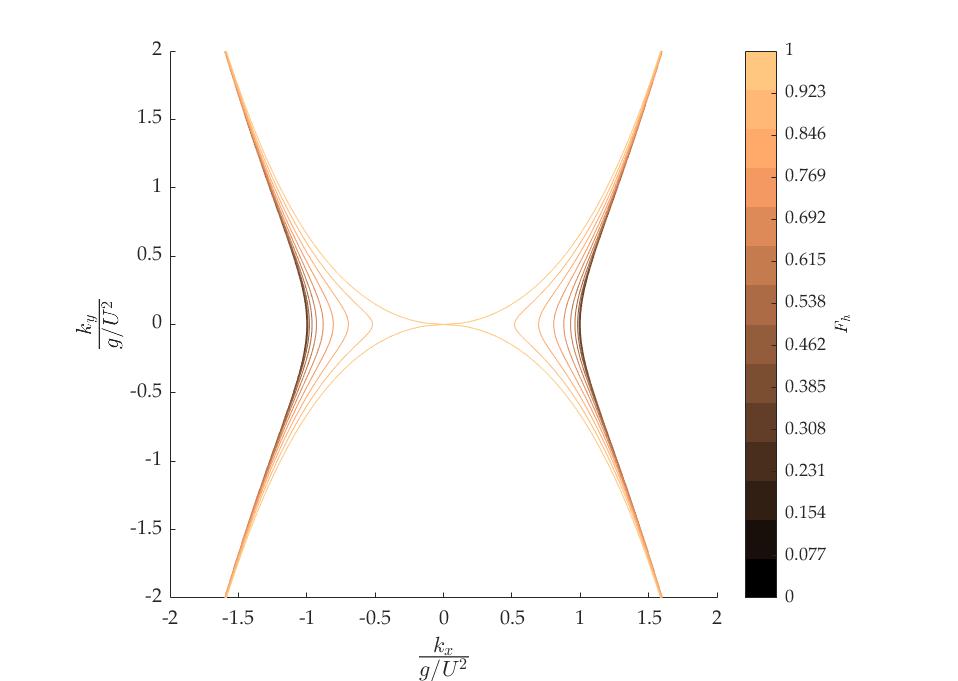
\[U^2k^2_x-g\sqrt{k_x^2+k_y^2}\tanh{h\sqrt{k_x^2+k_y^2}}=0\]with $h$ being the water depth. When \(kh>>1\), the results reduce to the deep water relations. To predict the wavelength, the value of $k_x$ at $k_y=0$ is computed by
\[U^2k_{c,x}^2-gk_{c,x}\tanh{hk_{c,x}}=0\]where $k_{c,x}$ is the cut-off wavenumber. The transverse wavelength is then $\lambda=2\pi/k_{c,x}$. The number of cells we wish to distribute per wavelength are specified in the Methods section through the property Cells/$\lambda$. Shallow water effects are accounted for only when the relevant tickbox is checked. It should be kept in mind that shallow water effects can have a singnificant effect on the $y^+$ values and may cause larger deviations than expected. An example of such deviations are reported in my upcoming paper on roughness effects on ship performance in confined waters.
Click here to see the full wavenumber plane for varying depth Froude numbers $F_h$
User interface
Click here to view the app user interface.
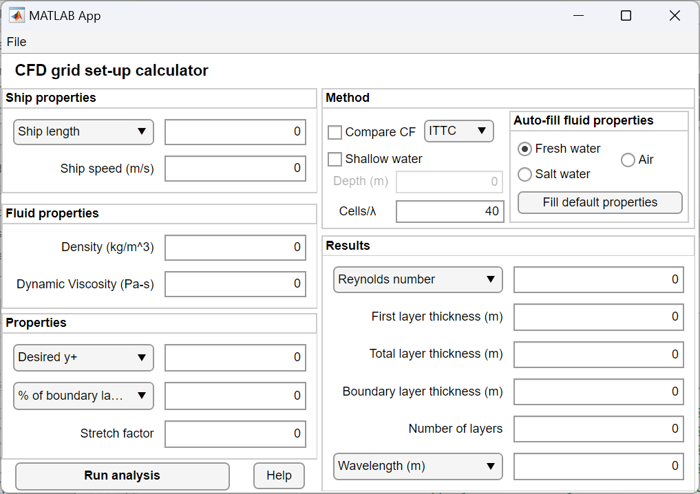
Controls
- The Help button opens this page
- The ‘Compare CF’ tickbox causes the Run analysis button to display the results from all methods to predict $C_f$ in the command window. Note that doing so requires the calculation of the Schoenherr line which is solved numerically for $C_f$ making the predictions a bit slower.
- The ‘Fill properties’ tickbox enters the fresh/salt water properties at 15 °C.
- The ‘Shallow water’ tickbox enables the Depth field and changes the calculation of the cut-off wavenumber $k_{c,x}$ from $g/U^2$ in deep water to the foruma shown in Equation 7. When this setting is enabled, $k_{c,x}$ is solved for numerically making predictions a bit slower.
Properties according to the ITTC:
| Property | Fresh water | Salt water | Air | Units |
|---|---|---|---|---|
| Density | 997.561 | 1026.021 | 1.18415 | \(kg/m^3\) |
| Dynamic viscosity | 0.00088871 | 0.00122 | 1.85508E-5 | \(Pa-s\) |
Changing the water temperature
The temperature may be set at any value between 0.1 °C and 50 °C at 0.1 °C increments to determine the density and viscosity of the fresh water or salt water. The menu can be accessed by right-clicking anywhere in the ‘Auto-fill fluid properties’ section. Full details can be found on the ITTC webpage.
Recording outputs
The ‘File’ menu can be used to trigger continous recording of all data shown in the command window. When prompted to create a file for recording the outputs, use .txt, .rtf or any other editor extension. The same menu can be used to switch logging off, or using the Exit option under the ‘File’ menu. Closing the app otherwise will not disable logging. Use diary off to disable logging manually.
Visualising layer distribution
The placement of cell centers and vertices in terms of their y+ allocation may be viewed by right-clicking the Run button. All fields in the inputs sections must be filled prior to triggering this setting.
Download and install
The app may be downloaded here, and installed by navigating to the MATLAB Apps ribbon.
It is possible to choose the desired \(y^+\) or the number of layers if known in advance. In the latter case, the \(y^+\) is computed in place of the number of layers. These settings may be changed through the dropdown menus in the Grid properties section. Similarly, when the first layer thickness is specified, the output field displaying the first layer thickness shows the achieved \(y^+\) instead.
Wishlist and planned updates
- Update user guide to include free surface mesh recommendations.
- Allow full wavenumber spectrum prediction capability.
- Compute dimensionless cut-off wavenumbers and wavelengths.
- Compute wavelengths with arbitrary direction.
- Incorporate free surface mesh recommendations in command window logging.
- Get in touch to suggest other capabilities.
Known problems
- the ‘First layer thickness’ label cannot revert once changed to ‘Achieved y+’.
Last update: November 9th 2022
- Update 3:
- Integrated free surface mesh recommendations (x-y) directions only.
- Integrated shallow water theory in wavelength prediction.
- Fixed bug that showed half of the first layer thickness under certain conditions
- Update 2:
- Added layer visualisation ability
- Added command window logging
- Update 1:
- Set automatic density and viscosity filling
- Added first layer thickness calculation capability
- Allow switching between Reynolds and Froude numbers in outputs